Millimeter-wave Intermodulation Distortion (IMD) Measurements

ME7838A Family

Abstract

While intermodulation distortion measurements are common at microwave frequencies, they are performed less often at mm-wave frequencies sometimes because of the complexity in setting up the measurement or because of hardware availability. The ME7838A family (broadband or waveguide band) has a number of features to make this process easier and to enable IMD measurements to 125 GHz and beyond.

1. Introduction

IMD has been a valuable measurement tool for specification conformance testing, predicting system performance based on component behavior, and general device and subsystem modeling (e.g., [1]-[3]). As demanding applications proliferate at mm-wave frequencies, this type of characterization information is increasingly needed but has sometimes not been obtained because of difficulties in performing the measurement at those higher frequencies. Among the challenges

• Two sources with adequate power control and offset frequency control combinable so that residual IMD products are not generated that could interfere with the measurement.
• A sufficiently linear receiver so that receiver IMD products do not dominate those of the DUT.
• A simple enough, yet flexible user interface that allows one to perform the needed measurement without too much complexity.
  
  

Previous broadband and mm-wave systems have had some issues with all of these categories including high expense in getting the second tone and the inability to control it well, the lack of adequate power control, the re-modulation of sources producing spurious products, relatively poor linearity of the receivers and user interfaces that were too limiting.

This note will explore the use of the ME7838A system for making these measurements in banded mm-wave and broadband settings: how the measurements can be setup, how the equipment is configured, how calibrations are performed, and the possibilities for more advanced measurements.
Some terms and definitions that will be used in this note (basic diagram in Fig. 1):

• IMD product
  • This is a distortion product created by the DUT (or sometimes the measurement system) by mixing multiples of the incident 2 tones used in this note. If the two tones are at f1 and f2 (f2>f1), the 3rd order products are at 2f2–f1 and 2f1–f2. The 2nd order products are at f2+f1 and f2–f1. The 5th order products are at 3f2–2f1 and 3f1–2f2 and so on. More of these details are discussed in, for example, [1]-[3].
• Upper product and lower product
  • If the product is above the two input tones in frequency, it is often called the ‘upper product’. Similarly, the product below the two main tones in frequency is called the ‘lower product’.
• Combiner
  • The two tones must be combined before feeding the DUT, usually with a passive network such as a directional coupler, a hybrid coupler, a resistive splitter, a Wilkinson combiner.
    

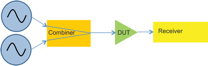
Figure 1. A generic IMD measurement setup is shown here to help introduce terminology. The two sources on the left generate signal tone1 and tone 2 which are combined before being fed to the DUT. The receiver measures outputs at tone1 and tone2 frequencies as well as at the frequencies of the IMD products of interest.

2. Hardware setup and configuration

The basic intermodulation distortion setup consists of sources providing 2 tones, a combining network, and a receiver. In the ME7838A system, small 3743A modules form the final interface for the sources and receivers so that a compact setup is possible. A second source is required to provide the second tone and, for the examples in this note, an external synthesizer under GPIB control will fulfill that role in conjunction with a third 3743A module. The setup is shown in Fig. 2. One may ask how the third module is powered and controlled. As shown in Fig. 3, the 3739B test set (part of the ME7838A system) has an auxiliary power connector that is used for this third module and provides power and control synchronized with the control for the module for tone 1 (normally from the internal source in the VNA).

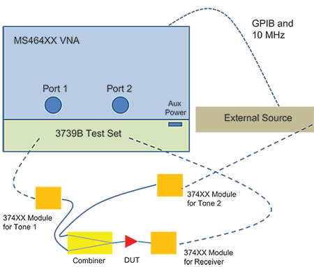
Figure 1. The setup configuration to be used in the examples of this note is shown here.

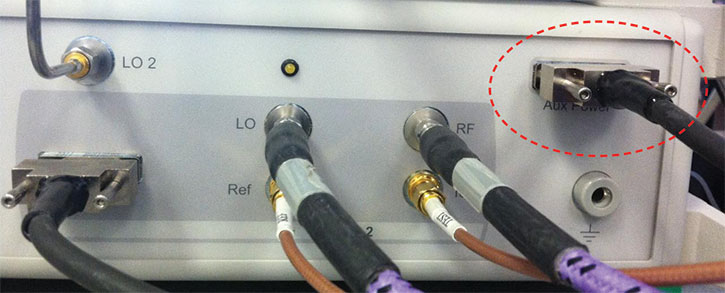
Figure 1. The front the 3739B test set is highlighted here to show the auxiliary power connector for the tone 2 module.

Generally, the receiver is the module connected to port 2 of the VNA so all of the measurements discussed in this note will be based on b2/1: the test channel on port 2. Other receiver paths can, of course, be used.

One remaining major item in Fig. 2 is the combining network. A variety of options are available including Wilkinson combiners, Lange couplers, directional couplers, and resistive splitters. Any of these can work if of the appropriate bandwidth although isolation between the source ports should sometimes be considered in very high dynamic range (very low IMD product) scenarios. The usual issue is that the leveling loops of the two sources can interact and cause spurious IMD products at the combination stage but the ME7838A leveling system is highly buffered so that high isolation is usually not needed down to –100 dBm product levels or lower. Contact Anritsu if assistance is needed in selecting a combiner for a given application.

Sometimes additional padding at the receiver input may be needed if the DUT output power is high. The 3743A receivers are highly linear so the requirements on level are not as stringent as with some other mm-wave receivers in the past but it is still possible to drive them hard enough that residual IMD products are generated. Main tone levels at the 3743A module of about –10 dBm are often ideal for maximum IMD dynamic range although levels above 0 dBm can be used (receiver IMD generation may get to –60 dBm) as can lower main tone levels (the receiver noise floor may limit the IMD level near –100 to –110 dBm). If additional pads or pre-amplifiers (make sure the pre-amp is of sufficiently good linearity), they should be attached to the receiver module for receiver calibrations discussed in the next section.

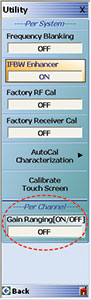
One other general configuration item has to do with the MS4640A IF system. This highly linear IF chain incorporates automatic gain control for improving dynamic range even more when in regular S-parameter modes but it can trigger gain too early if many other products are present within its bandwidth. It is thus sometimes helpful to disable this automatic gain ranging, particularly when the offsets are small. A general rule of thumb is to check the IMD products with gain ranging off and then enable it. If there is a rise in the data when gain ranging is enabled, then gain ranging should be turned off. The menu for controlling this function is under System/Utility and is shown in Fig. 4.

Fig. 4. The system/utility menu is shown here to highlight how gain ranging can be turned on or off. It is on by default but should be turned off if small offset products are interfering

3. Instrument configuration

Before proceeding with configuration details, it is helpful to consider what kind of measurement is desired (schematically shown in Fig. 5):

• CW tones (like a spectrum analyzer display where the tones and products are simultaneously visible, or a power sweep configuration)
• Swept with constant offset (the two tones move in frequency separated by a constant frequency offset). Generally a product level is plotted versus tone frequency.
• Swept offset (one tone is CW and the other tone moves relative to it, or both tones moves away from each other). Generally a product level is plotted versus the offset frequency.

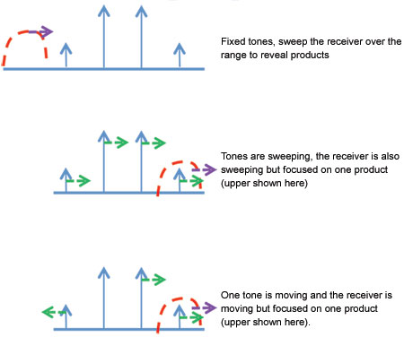
Figure 5. Three IMD measurement types are shown schematically here. The differences are in how the tones are moving (if at all) and where the receiver is looking (red dashed window).

The user-interface settings for these cases are slightly different but all are easily entered. The calibrations for all are very similar and will be covered in the next section. The Multiple Source Setup screen is used for all of these measurements and the relevant aspects will be discussed here (additional information is available in the MS4640A Measurement Guide [4]). For all of these examples, we will use external source 1 as our second tone and its 10 MHz reference will be synched to that of the MS464XX as suggested in Fig. 2.

3.1 CW measurements (spectrum analyzer-like display)

The central idea in this measurement is that the two tones will be set at CW frequencies and the receiver frequency will be swept over any product frequencies of interest. To speed up the measurement, segmented sweep can be used so one only measures at frequencies where products can be. The main multiple source setup screen is shown in Fig. 6 for this configuration and one can see that the internal source (for tone 1) and the external source 1 (for tone 2) are checked for CW and their frequencies are entered (examples of 94 and 94.1 GHz are shown here). The receiver and receiver source equation are left in their default states as these will be sweeping. We might want to sweep over 90-100 GHz so the band was defined with those limits (but much tighter or wider limits could have been entered since we will look only over < 1 GHz to see 9th order products and below).

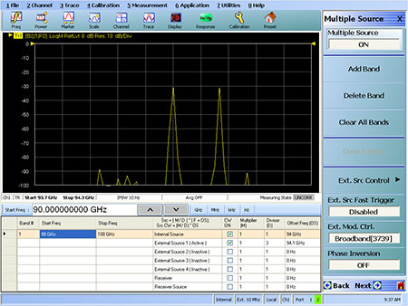
Figure 6. A multiple source screen for a 94 GHz CW IMD measurement is shown here.

The divisor shown for the external source may cause some questions. Since the 3743A module is being used and is under control of the 3739B test set, its multipliers are automatically activated based on the frequency. The rules are

54.000000001 GHz to 80 GHz: set the divisor to 2 for the external source

80.000000001 GHz to 120 GHz: set the divisor to 3 for the external source

120.000000001 GHz to 125 GHz: set the divisor to 4 for the external source

If one just entered the numbers above, one may have seen red exclamation marks on the left indicating erroneous entries. This is because the system must be informed that the 3743A modules are being used. As shown in Fig. 7, select the external module control button and enable broadband (or banded mm-wave depending on the model of instrument being used, the mm-wave option on the left will be discussed more in a later section) and enable the band as shown. For these mm-wave measurements (> 54 GHz), both source and receiver should be selected since the 3743A modules will be in use for both sides. An additional selection here is the source leveling choice. This determines if IF or RF (detection in the multiplier chain) leveling will be used. The IF leveling has more range and accuracy but is limited to frequency deviations between source1 and receiver of about 200 MHz (the setting shown would likely not be used for the setup of Fig. 6, RF leveling would be selected because of the potential sweep range). If a larger tone spacing is used, RF leveling must be selected for reasonably accurate power control. For more information, see the MS4640A measurement guide [4]. In both cases, the detection points in the 3743A modules are sufficiently buffered that self-modulation should be minimal and a large dynamic range will be available.

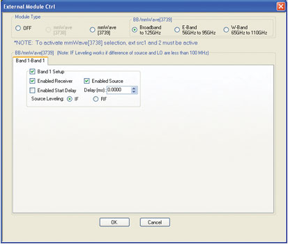
Figure 7. The external module control dialog is shown where the system is informed that the 3743A modules are being used for the IMD measurement.

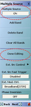
Figure 8. The buttons required for finishing the setup are highlighted here.

Once all these entries have been completed, select DONE on the main menu as suggested in Fig. 8 and activate multiple source mode by clicking ON.

As mentioned earlier, one may want to use segmented sweep to save measurement time by only making measurements where the products may land. In addition, one can customize the setup so that a lower IF bandwidth is used on the product measurements (for a lower noise floor and higher IMD dynamic range) than on the tone measurements. Under the sweep menu of the MS4640A, the frequency-based segmented sweep table can be entered. Two example setups are shown in Fig. 9 for measuring only the 3rd and 5th order products. The first is the absolute fastest in that only 6 points are measured. The second is also fairly fast (only 30 points) but creates a more easily interpreted display and allows one to gauge the level of the noise floor relative to the product levels. Note how the by-segment selection of IF Bandwidth is used in these example setups to help further optimize measurement time.

The tone power level must be selected as part of the measurement. The internal source in mm-wave bands has range down to ~ –60 dBm for even the lowest power devices. Tone 2 range will be set by the external source in these examples but can often approach the same range.

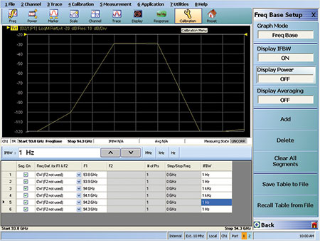
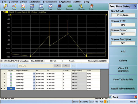
Figure 9. Two example segmented sweep setups for this measurement class are shown here. The first is the fastest. The second takes some additional measurements but provides more display information (such as the noise floor level).

3.2 Swept measurements with fixed offset

The swept measurements are a natural extension of what was discussed in section 3.1 and the external module control and completion steps are exactly the same. The difference now is that the CW checkboxes will be unchecked and we want both tone 1 and tone 2 moving but with a constant offset frequency. This is suggested in Fig. 10 where a 50 MHz offset frequency was selected. The receiver frequency must also be changed to force the system to look at a given product (different channels can be used to look at different products as will be shown in a later example). Here the offset is set to 100 MHz to look at the upper 3rd order product. A setting of –50 MHz would be used for the lower 3rd order product, +150 MHz for the upper 5th order product and so on. Note that the receiver source and receiver equations are set to the same value. This ensures that receiver calibration indexing will be correct as will be discussed shortly.

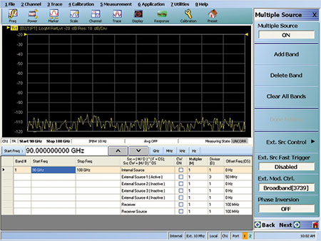
Figure 10. The multiple source setup screen for a swept measurement with fixed offset is shown here. The upper product is being measured with the settings shown.

Unlike in section 3.1, there is no speed advantage in using segmented sweep but it can, of course, be used if certain tone frequencies or frequency ranges are of interest.

While it is sometimes desired to view IMD product amplitudes in absolute terms (dBm), it is also often desired to look at them relative to the main tone level (dBc terms). This can be easily done using trace math and is illustrated in Fig. 11. Go back to multiple source setup and change the receiver and receiver source equations to the default 1/1(f+0)…this tells the receiver to follow tone 1 (which has the same equation). Select DONE and the frequency range of interest on the frequency menu….the plotted result of b2/1 is the absolute tone 1 power. Store this to trace memory (Display menu) and select Data-divided-by-Memory…this normalizes the result to tone 1 power. Now return to the multiple source menus and change the equations back to something like Fig. 10 (using the receiver offset corresponding to the product of interest) and click DONE. The plotted result on b2/1 is now the product in dBc terms relative to tone 1. Tone 2 could have also been used by changing the first step to have the receiver equation mimic the external source 1 rather than the internal source.

• STEP 1: Configure multiple source setup for the receiver to follow tone 1 (shown here) or tone 2.
• STEP 2: Store the result to memory (Display menu) and select Trace Math (data divided by memory)
• STEP 3: Go back to multiple source setup and configure like Fig. 9 (or equivalent for the measurement of interest). The displayed value is now in dBc terms
  

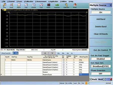
Figure 11. The process for a relative product measurement is delineated here.

3.3 Swept offset measurements

The process for this measurement class is very similar to that seen in section 3.2. The difference is again in how the sources are configured. A multiple source setup for this measurement is shown in Fig. 12. Here the tone 1 source (internal synth) is parked at 94 GHz and tone 2 is allowed to move from an offset of 100 kHz to 10 MHz. The band definition in this case was changed so that the x-axis of the display can read-out offset rather than absolute frequency. A setup for the latter display preference is shown in Fig. 13.

Figure 12. A multiple source setup for a swept offset measurement is shown here. The band definition was configured so the offset frequency would be the x-axis of the plots.

Figure 13. The same measurement of Fig. 12 is reconfigured here so the X-axis will display the tone 2 frequency.

The receiver equations may appear confusing at first in Figs. 12-13 but the reasoning is quite simple: all of the sources and receivers are defined by an easy linear relationship with the x-axis frequency (labeled F on the screens). The internal source is constant and the external source 1 relationship is straightforward. For the receiver in Fig. 12, we wish to have the receiver look at 2*x–axis value above 94 GHz. Since the equation is formed as (M/D)*(F + offset), we need M=2 and D=1 (so we get twice the tone spacing as the net position for the receiver) which forces the offset to be 94/2=47 GHz. For the receiver in Fig. 13, we want the receiver to be at 2x the delta between F and 94 GHz added to 94, or equivalently 2*(F–94)+94=2*F–94=2*(F–47 GHz). Here M=’multiplier’, D=’divisor’, OS=offset and F is the x-axis frequency.

The same trace math-based normalization scheme discussed in section 3.2 can be used for this measurement. Note that at very low offset frequencies (<1 MHz), the phase noise skirts may still be noticeably present at the product locations and can reduce dynamic range. A further reduction in IF bandwidth can help sometimes in this case but a smaller offset than is needed for the measurement application should normally not be used for this reason. This concept is shown in Fig. 14. In the mm-wave ranges, since the source multiplier numbers are larger, this can sometimes be a larger issue than at lower frequencies but the MS4640A source cleanliness should minimize the problem. For all of the measurement classes, there are certain offsets where system spurious products can also reduce dynamic range (e.g., 10 MHz is the system reference frequency). Slight changes to the offset or frequency list can sometimes help (e.g., use 9.999 MHz instead of 10 MHz).

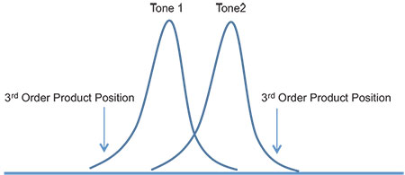
Figure 14. The issues present in small-offset measurements are schematically shown here. As the tones get closer together, the location where the product needs to be measured moves further up the phase noise skirts of the source and can reduce the available dynamic range.

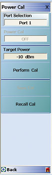
Figure 15. The power calibration submenu is shown here.

For the ME7838A system, two different power sensors are typically used: the SC7770 for frequencies below 70 GHz and the W8486A for frequencies between 70 and 125 GHz. The system will automatically access the GPIB address for the given power meter (settings are on the remote submenu but are 13 and 15, respectively, by default) and will ask for a power sensor change if the frequency range of the calibration crosses 70 GHz. The target power shown in Fig. 15 is to help the system speed up its calibration by implicitly providing a way of entering the loss between the VNA test port and the desired reference plane. Suppose the desired power is –10 dBm but the combiner and cabling network has about 5 dB of loss. Then one would enter –10 dBm as the target (since that is what the VNA will search for) but –5 dBm can be entered on the main power menu prior to executing the calibration to speed up the search. The internal source has a controllable power range down to ~–60 dBm in mm-wave bands to help handle even very low power devices.

The external synthesizer has its own flat power calibration algorithm that can be executed from the synthesizer front panel using the same power meter. One must leave multiple source mode so that the synthesizer can be operated from the front panel to do this calibration. If this calibration is active on the synthesizer, it will be used when the synthesizer is back under multiple source control for the IMD measurement.

The receiver calibration can be done with the uncombined signal or with the combined signal port after a power calibration has been done. The purpose is to transfer a known power level to the receiver so that b2/1 readings can be interpreted as dBm. This calibration should be done with the receiver tuned to the internal source frequency or in regular 3739B mode and a thru should be connected from the power calibrated plane to the desired receiver reference plane (where the DUT output will be connected). For the IMD measurements in this note, only the Test–port2 receiver calibration needs to be done. The lower level submenu for this is shown in Fig. 16 along with the result after the calibration was performed at –10 dBm. The upper level menu is also shown in Fig. 16.

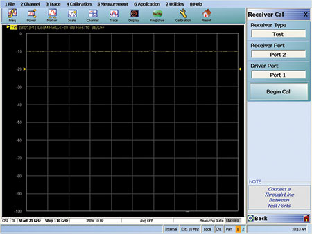
Figure 16. The receiver calibration menus and results are shown here.

The power level of the receiver calibration is not critical as long as the receiver is linear at that level (generally anything below +10 dBm for the 3743A modules) and the driving power accuracy is good at that level. If the driving power is from the port 1 3743A module, this level should normally be –5 dBm or less and one can rely on the factory ALC calibration in many cases. If a different driving reference plane is used (i.e., at the combiner output) or more accuracy is desired (sub 1 dB), then a power calibration as discussed above should be used. For more information on receiver calibrations, see the Measurement Guide [4].

In the multiple source setup screens earlier, one of the equations was labeled ‘receiver source’. This equation provides an index into the receiver calibration table. Normally this will be set equal to the receiver equation. The only exception is when there is a frequency conversion stage between the desired reference plane and the receiver frequency plane. This sometimes can happen in higher mm-wave frequency bands discussed later in this note and in the Measurement Guide [4].

5. Example measurements

To illustrate some of these points, a series of measurements were made using the setups described and a W-band amplifier as the DUT. This physical setup is shown in Fig. 17. The module labeled ‘Tone 1’ is connected to port 1 of the 3739B test set and the module labeled ‘Receiver’ is connected to port 2. The ‘Tone 2’ module is connected to an external MG369XX synthesizer and the module power/control comes from the Aux Power connector on the 3739B test set discussed earlier.

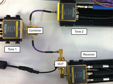
Figure 17. The physical setup for some example measurements is shown here.

The first measurement is a CW one using the setup described in Fig. 6 and the results are shown in Fig. 18 using a segmented sweep configuration similar to that discussed previously. This is a relatively low power amplifier so the output tone levels are low (around –20 dBm) with the 3rd order products around –82 dBm, the 5th order products around –90 dBm, and the noise floor of the measurement in the –100 dBm range. These measurements were made with a 30 Hz IFBW on the product measurements so it could be reduced further if a lower noise floor level was required.

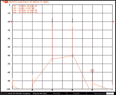
Figure 18. The results of an example CW measurement are shown here.

A swept measurement (similar to that described in Fig. 10) was also performed and the results shown in Fig. 19. A normalization like that described in Fig. 11 was used (notice the ‘[D/M]’ annunciator in Fig. 19) so the results are plotted in dBc terms. A constant offset of 50 MHz was used here as the tones swept. The frequency dependence of the result shows why a swept result with mm-wave devices can present more information than just a few CW measurements.

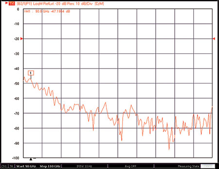
Figure 19. A swept measurement result is shown here in dBc terms (3rd order product).

A swept offset measurement was also performed (setup like that in Fig. 11) and the results are shown in Fig. 20 for an offset range of 100 kHz to 10 MHz. Tone 1 was kept fixed at 94 GHz. This time two channels were used to look at the upper product (left, channel 1) and the lower product (right, channel 2). There is some structure with offset frequency and the asymmetry between the products differs with offset frequency. This can be an indication of memory effects in the device (due to IMD products circulating in the bias network, interacting with thermal time constants, etc.) and can be a useful characterization tool as has been discussed in the literature (e.g., [5]-[7]).

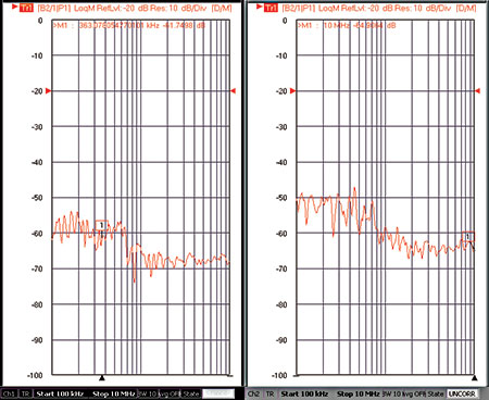
Figure 20. An example swept offset measurement is shown here for both the upper product (right) and lower product (left).

6. Uncertainties

• Receiver linearity and residual IMD products.
  • Due to the linearity of the 3743A receivers, this is usually not a dominant factor unless the incident levels are too high. With –10 dBm incident tones, the residual products are generally < –100 dBm. Thus if one is measuring –80 dBm tones from the DUT, the receiver induced uncertainty would be under 1 dB.
• Source linearity and residual products
  • If the sources communicated with each other, there could be remodulation and spurious IMD generation on the source side. Because of the buffering the 3743A modules, this effect should be insignificant for product levels above –100 dBm with the use of even a relative low isolation (<10 dB) combiner.
• Receiver calibration accuracy
  • If reading out the product values in dBm or converting to an intercept value, the absolute power accuracy is important and is dependent on the power calibration behind it. Using the power calibration techniques discussed, this uncertainty should normally be under 0.5 dB.
• Return loss
  • Match interactions between the combiner and DUT or between DUT and receiver can have impacts on the order of the products of the reflection coefficients (in linear terms). Padding on the receiver or combiner (before the reference planes) can help reduce these effects if dynamic range allows.
• Noise floor
  • The noise floor of the instrument can be the limiting factor in some cases but the high dynamic range of the 3743A modules helps in this regard. In a 10 Hz bandwidth, the noise floor is typically in the –110 dBm range and the use of a lower IFBW can help further.

7. Higher mm-wave frequencies

If one needs to perform IMD measurements above 125 GHz, higher frequency mm-wave modules are available (to THz range). Most of the concepts discussed in this note still apply with the following comments:

• In the multiple source setup menu, a different external module control setting must be used and this is shown in Fig. 21. The selections have the same meaning as for the 3743A modules except for the common offset selection and the overrange field which are used for certain higher frequency module frequency plans. See the Measurement Guide for more information [4].
  

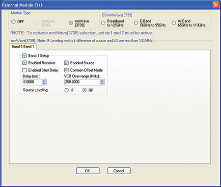
Figure 21. The external module control panel (within multiple source setup) is shown here for mm-wave module selection above 125 GHz.

• The appropriate divisors must be entered in the equation fields for the module being used. Unlike the 3743A version, the internal source and receiver divisor will no longer be 1 (they will be more like the 1/3 used for the external source in the examples; the system handled the divisors automatically for the 3743A).
• Power measurement and calibration becomes more challenging as fewer power meters are available and automatic control behaves differently. See the measurement guide [4] or contact Anritsu for more information.

8. Conclusions

The setup requirements and procedures for performing a variety of IMD measurements with the ME7838A system using the 3743A modules have been presented including absolute and relative product measurements in CW, swept, and swept offset configurations for arbitrary product orders. The configuration flexibility coupled with the high linearity and wide power control of the system can help lead to a wide range of high performance mm-wave IMD measurements.

Note: The SM6499 and SM6527 mmwave modules are banded versions of the 3743A mmwave module operating in the E band and W band respectively. The ME7838A system may be configured with either SMxxxx module and still perform the IMD measurements described in this application note.